This work is licensed under a Creative Commons Attribution-ShareAlike 3.0 Unported License. This means that you are able to copy, share and modify the work, as long as the result is distributed under the same license.
Integrated assignment: g:Profiler/EnrichmentMap
By Veronique Voisin
Goal
Familiarize yourself with g:Profiler and GSEA as well as with Enrichment Map Cytoscape app.
Background
Esophageal adenocarcinoma (EAC) is a devastating disease with rising incidence and a 5-year survival of only 15%. The single major risk factor for development of EAC is chronic heartburn, which eventually leads to a change in the lining of the esophagus called Barrett’s Esophagus (BE).
Specimens were collected from patients with normal esophagus (NE) and Barrett’s esophagus (BE). RNA was extracted from these samples and expression profiling was assessed using Affymetrix HG-U133A microarray PMID:24714516. Differentially expressed genes between BE and NE were determined.

Data processing
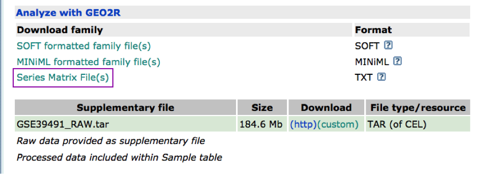
The Affymetrix data are stored in the Gene Expression Omnibus (GEO) repository under the accession number GSE39491 PMID:24714516. The RMA (Robust Multichip Average) normalized data were downloaded from GEO and further processed using the Bioconductor package limma to estimate differential expression between the groups. The results of the limma t-tests were corrected for multiple hypotheses using the Benjamini-HochBerg method (FDR).
For g:Profiler, genes with a FDR <=0.0001 and a logFC of 2 were selected to create the gene list. For GSEA, a rank file has been created by ranking the genes from the highest t statistics value (up-regulated in BE compared to NE) to the lowest t values (down-regulated in BE compared to NE). The code used to process the data is available from the course wiki. Please feel free to adapt it and use it with your own data.
Our goal is to use the gene list from the BE specific genes to familiarize ourself with g:Profiler and then to download the BE and NC lists as an Enrichment Map output. In the last step, we will create a network using the BE and NC g:Profiler outputs.
PART 1
-
Open g:Profiler
-
In Options, check Significantly only, No electronic GO annotations
-
Choose the databases: GO BP and Reactome.
-
Set minimum size of functional category to 3 and maximum to 500. Set 2 for the Size of query/ term intersection.
-
Set Benjamini-Hochberg as the significance threshold.
-
Run analysis of the genes differentially altered between BE and normal: BEonly_genelist.txt.
-
What is the most significant GO:term? What is the p-value for this GO:term?
-
Is this p-value already corrected for multiple testing? What type of correction is used for your current analysis?
PART 2
- Re-run the analysis with User p-value threshold set to 0.0001. What has been changed?
PART 3
An important feature of g:Profiler is an ability to work with sorted or ranked lists. The top of such a list is given more weight in determining the functional connections to GO:terms and/or pathways. Our gene list was initially sorted by the FDR value based on the significant differential expression.
-
Open g:Profiler in a new window and paste genes from BEonly_genelist.txt.
-
Use same options as part 2 (User p-value threshold set to 0.0001) and select also Ordered query.
-
Do you seen any changes in the output in comparison to the analysis of the unordered gene list (PART 2)?
PART 4
Now we have to generate an output from the enrichment analysis and save it in appropriate format for EnrichmentMap. Please, change the output type to Generic Enrichment Map (TAB).
Run it using options used in PART 1. Download data in Generic Enrichment Map (GEM) format. We will need this file for Enrichment map.
PART 5
Generate and save the Generic Enrichment map for genes in NConly_genelist.txt. It contains the genes specific of the normal tissue samples. Run g:Profiler with this list using same options as in PART 4 selecting Generic Enrichment Map (GEM) format as output type. We will need this file for Enrichment map.
PART 6
The EnrichmentMap Cytoscape app allows users to translate large sets of enrichment results to a relatively simple network where similar GO:terms and/or pathways are clustered together.
We will use Enrichment map app to visualize the outputs from g:Profiler and compare 2 enrichment analyses.
-
Open Cytoscape
-
Go: Apps > EnrichmentMap > Create Enrichment Map
-
Let’s create an EnrichmentMap for the pathways that were enriched by the genes specific of the BE samples (as dataset1) and the genes specific of the NC samples (as dataset2) . Upload files into app and build the map. You can use the optional BE_vs_NE_expression.txt file.
-
If successful, you will see a network where each node represents a pathway and edge connects pathways with shared genes. Node size is proportional to the number of genes in this pathway, intensity of the node color represents the enrichment strength and edge weight - number of genes shared between connected nodes.
-
Try different layouts. For example: Layouts -> yFiles Layouts -> Organic; Move nodes around to be able to read the labels.
-
Using the search box (upper right corner of Cytoscape) find STEM CELL DEVELOPMENT node. When node is highlighted, expression profile of all genes included in this pathway appears in the Heat Map (nodes) viewer tab. Get familiar with the options provided by this panel. Save expression Set.
-
Click on any edge (the line between nodes). In the Table panel ( Heat Map (edges)) you should see a heatmap of all genes both gene-sets connected by this edge have in common
-
Select several nodes and edges. Heat Map (nodes) will show the union of all genes in the selected gene sets. Heat Map (edges) will show only those genes that all selected sets have in common.
-
Go to View -> Show Results Panel. Change q-value (FDR) as well as similarity cutoffs and see how the network changes. Redo the layout. Save the file.
What conclusions can you make based on these networks?
Nodes connected by green edges are BE (dataset1)
Nodes connected by blue lines are NE (dataset2)

PART 7: GSEA
-
Re-launch GSEA.
-
Run GSEA using the rank file that has been created from the differential expression test comparing BE vs NE BEvsNE_ranks.rnk and the pathway file Human_GOBP_AllPathways_no_GO_iea_May_24_2016_symbol.gmt. Use 100 permutations (do use 1000 permutations when you analyze your own data).
-
Create an EnrichmentMap.
-
Examine the results. Save the file.
