Answers to Integrated Assignment Day 2

Q1) How many total sample files do we have?

A1: There are two ways to do this:

• List and count the number of *.fasta files we have in our folder

ls *.fasta | wc -l

• Count the lines in the metadata file. Each row in the metadata file corresponds to one sample. Remember to subtract 1 as the first row contains the headers

wc -l metadata-file-for-osd-subset-210615.txt

There are 25 sample files.

Q2) How many sequences does the sample from OSD station 10 contain?

A2: Since we are dealing with fasta files we can do this by counting the number of “>” characters in the file using the grep command

grep -c “>” OSD10.comb.qc.masked.dedup.subsample.fasta

There are 100257 sequences.

Q3) How many samples of each type are there in each of the different Province code categories?

A3: Again we can use the metadata file for this. The prov_code is in column 12 in the file and we can use the sort and uniq commands to to get a count of each type.

cut -f 12 metadata-file-for-osd-subset-210615.txt | sort |uniq -c

There are 9 ARCT samples and 16 NWCS samples.

Q4) In the STAMP analysis of the Metaphlan results, do you see any separation in the samples when the PCA is coloured by Depth?

A4: No.

Q5) Do you see any separation in the samples when the PCA is coloured by the province codes? If so, describe which PC axis differentiates these samples.

A5: Yes, there is a slight separation between the Arctic samples and the Northwest Atlantic samples. The separation is seen in the PC1 vs PC2 and occurs partly along PC2.

Q6) In a “multiple group test” using ANOVA with no multiple test correction how many species are statistically significant?

A6: 4

Q7) How many are still significant in the “two group test” using White’s non-parametric t-test without and with Benjamini-hochberg FDR for multiple test correction?

A7: Without Benjamini-Hochberg FDR: 27. With: 23.

Q8) What are the top 3 Modules present in the 1m sample from the Bedford basin (station 152)?

A8: You can find this out from the kos.spf file that we generated. You can view the kos.spf file using less and manually count the column number where the OSD152 1m sample occurs. In this case it is 13.

less kos.spf

Now we will cut out that column (which contains the abundances pf the modules for OSD152 1m) and sort it based on the abundance values and list out the top 10 most abundant values

cut -f 13 kos.spf | sort -gr |head

Next we will take the top most abundant value (0.00419118 in this case) and grep the 1st column (which contains the pathway name) using this value

cut -f 1,13 kos.spf | grep 0.00419118

You can do the same for the top 3 abundance values.

The corresponding top 3 module names are as follows:

K07497: putative transposase

K00540

K00525: ribonucleoside-diphosphate reductase alpha chain

Q9) In the STAMP analysis of the Humann results using a two group test with no multiple test correction applied how many significant differences are seen between the Arctic and Northwest Atlantic samples?

A9: 645

Q10) What happens when the p-value cut-off is lowered to 0.01 for Q9?

A10: The significantly different modules decrease to 154

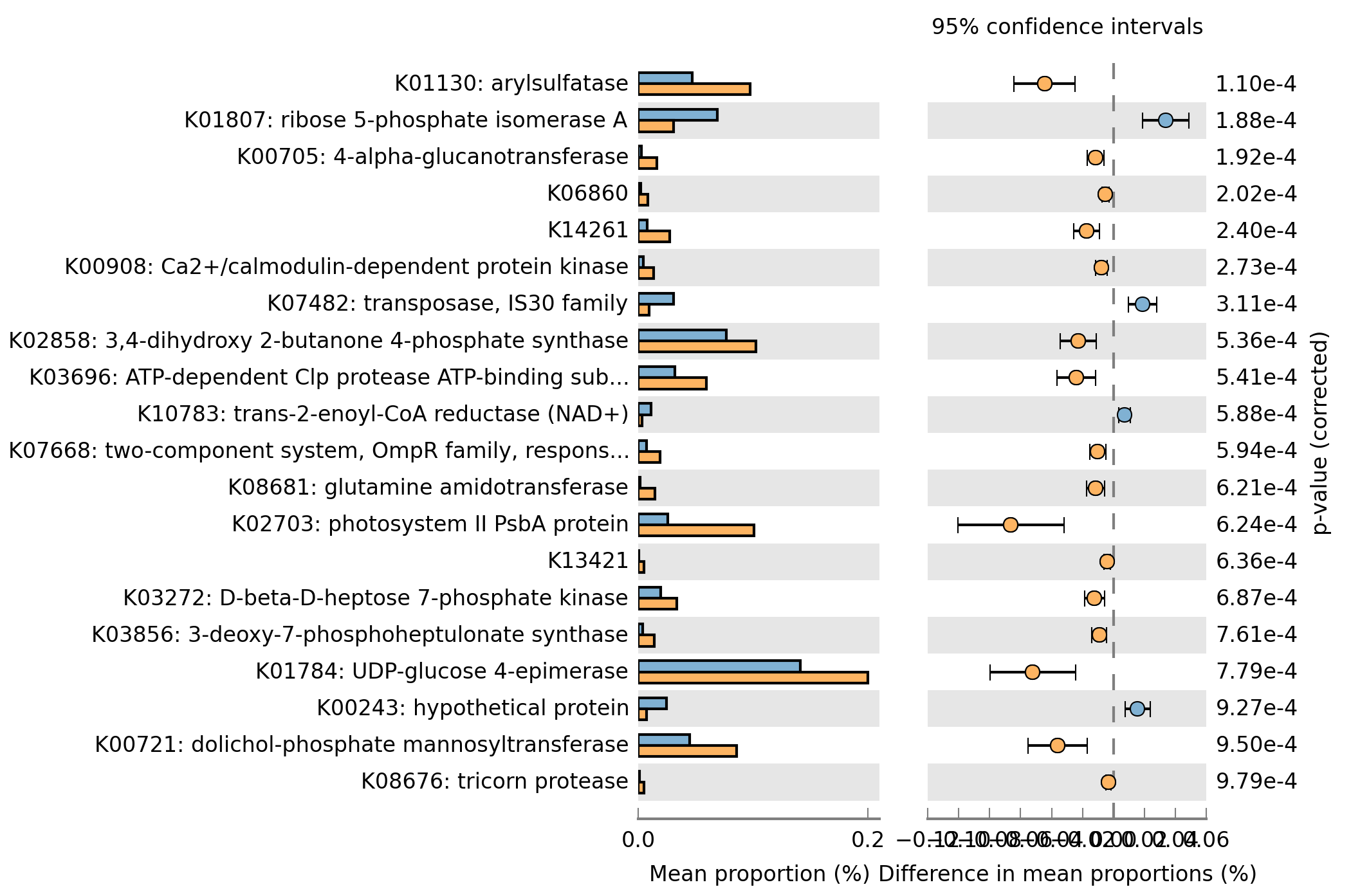
Q11) What is the most significantly different KEGG orthology group? What is the p-value for this KO?

A11: K01130: arylsulfatase. P-value: 1.10e-4

Q12) Change the p-value to 0.001 and create an “Extended error bar” plot and save the image as a .png using the File->Save Plot option.

A12: