Gene fusion visualization
Installation
The required libraries are in bioconductor and can be obtained using the biocLite function. You may not require this code block if you have already installed the libraries.
source("http://bioconductor.org/biocLite.R")

biocLite("GenomicRanges")
biocLite("ggbio")
biocLite("Gviz")
biocLite("BSgenome.Hsapiens.UCSC.hg19")
Load the required libraries.
library(ggbio)

## Loading required package: methods
## Loading required package: BiocGenerics
## Loading required package: parallel
##
## Attaching package: 'BiocGenerics'
##
## The following objects are masked from 'package:parallel':
##
##     clusterApply, clusterApplyLB, clusterCall, clusterEvalQ,
##     clusterExport, clusterMap, parApply, parCapply, parLapply,
##     parLapplyLB, parRapply, parSapply, parSapplyLB
##
## The following object is masked from 'package:stats':
##
##     xtabs
##
## The following objects are masked from 'package:base':
##
##     anyDuplicated, append, as.data.frame, as.vector, cbind,
##     colnames, do.call, duplicated, eval, evalq, Filter, Find, get,
##     intersect, is.unsorted, lapply, Map, mapply, match, mget,
##     order, paste, pmax, pmax.int, pmin, pmin.int, Position, rank,
##     rbind, Reduce, rep.int, rownames, sapply, setdiff, sort,
##     table, tapply, union, unique, unlist, unsplit
##
## Loading required package: ggplot2
## Need specific help about ggbio? try mailing
##  the maintainer or visit http://tengfei.github.com/ggbio/
##
## Attaching package: 'ggbio'
##
## The following objects are masked from 'package:ggplot2':
##
##     geom_bar, geom_rect, geom_segment, ggsave, stat_bin,
##     stat_identity, xlim

library(Gviz)

## Loading required package: S4Vectors
## Loading required package: stats4
## Loading required package: IRanges
## Loading required package: GenomicRanges
## Loading required package: GenomeInfoDb
## Loading required package: grid

library(GenomicRanges)
library(knitr)
Read the data
We will be working with predictions from deFuse. The output of deFuse is a tab delimited text file. This can be read with the read.table command.
results_url = "http://cbwmain.dyndns.info/Module4/packages/cbw_tutorial/gene_fusions/data/HCC1395/defuse/results.filtered.tsv"
data = read.table(results_url, sep="\t", header=T, stringsAsFactors=F)
Use the colnames function to take a look at the data provided by deFuse.
colnames(data)

##  [1] "cluster_id"                     "splitr_sequence"
##  [3] "splitr_count"                   "splitr_span_pvalue"
##  [5] "splitr_pos_pvalue"              "splitr_min_pvalue"
##  [7] "adjacent"                       "altsplice"
##  [9] "break_adj_entropy1"             "break_adj_entropy2"
## [11] "break_adj_entropy_min"          "breakpoint_homology"
## [13] "breakseqs_estislands_percident" "cdna_breakseqs_percident"
## [15] "deletion"                       "est_breakseqs_percident"
## [17] "eversion"                       "exonboundaries"
## [19] "expression1"                    "expression2"
## [21] "gene1"                          "gene2"
## [23] "gene_align_strand1"             "gene_align_strand2"
## [25] "gene_chromosome1"               "gene_chromosome2"
## [27] "gene_end1"                      "gene_end2"
## [29] "gene_location1"                 "gene_location2"
## [31] "gene_name1"                     "gene_name2"
## [33] "gene_start1"                    "gene_start2"
## [35] "gene_strand1"                   "gene_strand2"
## [37] "genome_breakseqs_percident"     "genomic_break_pos1"
## [39] "genomic_break_pos2"             "genomic_ends1"
## [41] "genomic_ends2"                  "genomic_starts1"
## [43] "genomic_starts2"                "genomic_strand1"
## [45] "genomic_strand2"                "interchromosomal"
## [47] "interrupted_index1"             "interrupted_index2"
## [49] "inversion"                      "library_name"
## [51] "max_map_count"                  "max_repeat_proportion"
## [53] "mean_map_count"                 "min_map_count"
## [55] "num_multi_map"                  "num_splice_variants"
## [57] "orf"                            "read_through"
## [59] "repeat_proportion1"             "repeat_proportion2"
## [61] "span_count"                     "span_coverage1"
## [63] "span_coverage2"                 "span_coverage_max"
## [65] "span_coverage_min"              "splice_score"
## [67] "splicing_index1"                "splicing_index2"
## [69] "transcript1"                    "transcript2"
## [71] "probability"
Many features and annotations are provided. We will primarily be intersted in the chromosome, strand, start and end annotations, and cluster_id which is the unique identifier assigned to each prediction.
We will concentrate on the EIF3K-CYP39A1 fusion. Filter the data for this fusion.
gene_names = c("EIF3K", "CYP39A1")
gene_names

## [1] "EIF3K"   "CYP39A1"

fusion = data[data$gene_name1 %in% gene_names & data$gene_name2 %in% gene_names,][2,]
fusion$splitr_sequence <- NULL
fusion

##     cluster_id splitr_count splitr_span_pvalue splitr_pos_pvalue
## 315    4311846          155        1.62879e-06         0.8150972
##     splitr_min_pvalue adjacent altsplice break_adj_entropy1
## 315         0.6862973        N         N           3.316957
##     break_adj_entropy2 break_adj_entropy_min breakpoint_homology
## 315           3.393843              3.316957                   6
##     breakseqs_estislands_percident cdna_breakseqs_percident deletion
## 315                              0              0.005789249        N
##     est_breakseqs_percident eversion exonboundaries expression1
## 315             0.001663894        N              Y       22357
##     expression2           gene1           gene2 gene_align_strand1
## 315        5935 ENSG00000178982 ENSG00000146233                  +
##     gene_align_strand2 gene_chromosome1 gene_chromosome2 gene_end1
## 315                  -               19                6  39127595
##     gene_end2 gene_location1 gene_location2 gene_name1 gene_name2
## 315  46620523         coding         coding      EIF3K    CYP39A1
##     gene_start1 gene_start2 gene_strand1 gene_strand2
## 315    39109735    46517541            +            -
##     genome_breakseqs_percident genomic_break_pos1 genomic_break_pos2
## 315                          0           39123318           46607405
##                           genomic_ends1
## 315 39114837,39116742,39123136,39123317
##                           genomic_ends2
## 315 46604219,46605715,46607405,46609900
##                         genomic_starts1
## 315 39114815,39116668,39123070,39123241
##                         genomic_starts2 genomic_strand1 genomic_strand2
## 315 46604188,46605566,46607231,46609900               +               +
##     interchromosomal interrupted_index1 interrupted_index2 inversion
## 315                Y                  -                  -         N
##     library_name max_map_count max_repeat_proportion mean_map_count
## 315      HCC1395             2                     0       1.176471
##     min_map_count num_multi_map num_splice_variants orf read_through
## 315             1             3                   1   Y            N
##     repeat_proportion1 repeat_proportion2 span_count span_coverage1
## 315                  0                  0         17       1.989058
##     span_coverage2 span_coverage_max span_coverage_min splice_score
## 315       1.947271          1.989058          1.947271            4
##     splicing_index1 splicing_index2                     transcript1
## 315               -               - ENSG00000178982|ENST00000591409
##                         transcript2 probability
## 315 ENSG00000146233|ENST00000275016    0.653798
The GViz package works best with UCSC style chromosome names. Convert the gene_chromosome1 and gene_chromosome2 fields.
fusion$gene_chromosome1 = paste("chr", fusion$gene_chromosome1, sep="")
fusion$gene_chromosome2 = paste("chr", fusion$gene_chromosome2, sep="")
fusion$gene_chromosome1

## [1] "chr19"

fusion$gene_chromosome2

## [1] "chr6"
Extract the chromosome and strand of the the fusion. Here the strand is referring to the strand of the genome, which is different than the strand on a gene which itself may be on the “-“ strand of the genome.
chromosome1 = fusion$gene_chromosome1
strand1 = fusion$genomic_strand1
Defuse predicts a fusion contig based on spanning and split RNA-Seq reads. The contig is a set of (potentially multiple) exons adjacent to the fusion boundary. The starts and ends of these exons are encoded in the genomic_starts1/2 and genomic_ends1/2 fields as comma separated lists.
starts1 = as.numeric(strsplit(fusion$genomic_starts1, ",")[[1]])
ends1 = as.numeric(strsplit(fusion$genomic_ends1, ",")[[1]])
starts1

## [1] 39114815 39116668 39123070 39123241

ends1

## [1] 39114837 39116742 39123136 39123317
Many plotting funcitons in R take GRanges (GenomicRanges package) objects containing information about the genomic regions to be plotted. We will encode the fusion exons as GRanges objects.
fusionexons1 <- GRanges(
  seqnames = chromosome1,
  ranges = IRanges(start = starts1, end = ends1),
  strand = strand1,
  group = rep("fusionexons", length(starts1)))
Plot a fusion using Gviz
We can plot the fusion exons in Gviz by creating a gene region track using the GRanges to define the exons and providing som additional information. Plot the track using the plotTracks function.
fusionTrack <- AnnotationTrack(fusionexons1, genome = "hg19", name = "fusion",
  groupAnnotation = "group", shape = "box", stacking = "dense")

plotTracks(list(fusionTrack))
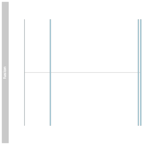
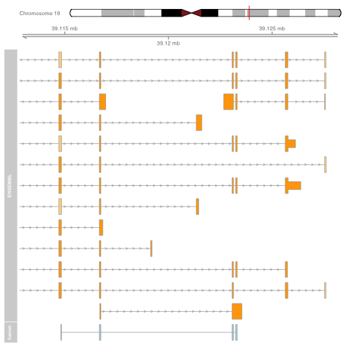
The plot shows the exons of the fusion, though in isolation the exons are not very interesting. Add an ideogram with IdeogramTrack, genomic location using GenomeAxisTrack, and ensembl gene models using BiomartGeneRegionTrack.
plot.start = min(starts1) - 2000
plot.end = max(ends1) + 5000

itrack <- IdeogramTrack(genome = "hg19", chromosome = chromosome1)

gtrack <- GenomeAxisTrack(genome = "hg19", chromosome = chromosome1)

biomTrack <- BiomartGeneRegionTrack(genome = "hg19",
  chromosome = chromosome1, start = plot.start, end = plot.end,
  name = "ENSEMBL")

plotTracks(list(itrack, gtrack, biomTrack, fusionTrack), from = plot.start, to = plot.end)
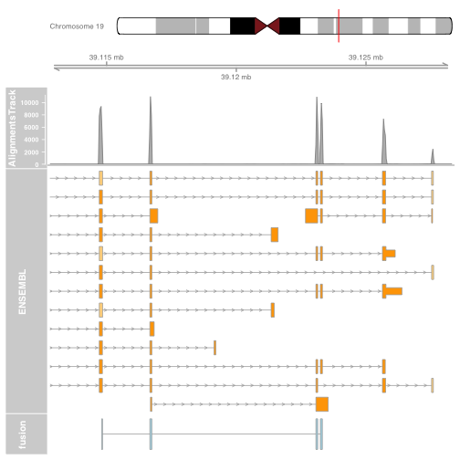
It is also possible to plot read alignments and coverage directly from a bam file using the AlignmentsTrack. The bam file should ideally have ucsc chromosome names to have the optimal compatibility with GViz. Set the sizes argument so that the alignments track doesnt take over the entire plot.
bam_url = "http://cbwmain.dyndns.info/Module4/HCC1395/rnaseq/genes/HCC1395_EIF3K.bam"
bai_url = "http://cbwmain.dyndns.info/Module4/HCC1395/rnaseq/genes/HCC1395_EIF3K.bam.bai"

bam_file <- basename(bam_url)
bai_file <- basename(bai_url)

download.file(bam_url, bam_file)
download.file(bai_url, bai_file)

alTrack <- AlignmentsTrack(bam_file,
  isPaired = TRUE, type = "coverage")

plotTracks(list(itrack, gtrack, alTrack, biomTrack, fusionTrack),
  chromosome = chromosome1, from = plot.start, to = plot.end,
  sizes = c(0.5, 0.5, 1, 3, 0.5))
Try other types of alignment plotting, by setting the type argument to “coverage”, “sashimi” or “pileup”. For sashimi plots, use type = c("sashimi", "coverage").
Visualizing the fusion break end
We will visualize the fusion break end using a highlight track overlayed on the fusion track.
Create the highlight track starting and ending at the fusion break end. Apply to the fusion track.
brkendTrack <- HighlightTrack(trackList = list(fusionTrack),
  chromosome = chromosome1, start = fusion$genomic_break_pos1,
  end = fusion$genomic_break_pos1,
  inBackground = FALSE, col = "darkred", fill = NA)
Plot the highlight track and gene model and ideogram tracks.
Note: The highlight should be plotted instead of the track its highlighting. Plotting the highlight track will plot the fusion track for you.
plotTracks(list(itrack, gtrack, alTrack, biomTrack, brkendTrack),
  chromosome = chromosome1, from = plot.start, to = plot.end,
  sizes = c(0.5, 0.5, 1, 3, 0.5))
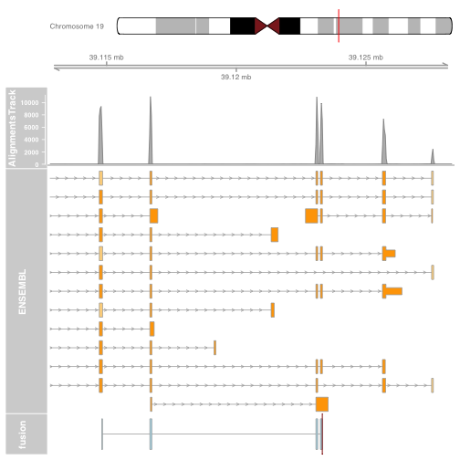
Plotting the fusion break end in the context of the gene models will now give us an idea for which intron of the gene harbours the associated genomic rearrangement breakpoint.
Plot the other end of the fusion
starts2 = as.numeric(strsplit(fusion$genomic_starts2, ",")[[1]])
ends2 = as.numeric(strsplit(fusion$genomic_ends2, ",")[[1]])
fusionexons2 <- GRanges(
seqnames = fusion$gene_chromosome2,
ranges = IRanges(
start = starts2,
end = ends2),
strand = fusion$genomic_strand2,
group = rep("fusionexons", length(starts2)))
fusionTrack <- AnnotationTrack(fusionexons2,
genome = "hg19", name = "fusion",
shape = "box", stacking = "dense",
groupAnnotation = "group")
brkendTrack <- HighlightTrack(trackList = list(fusionTrack),
chromosome = fusion$gene_chromosome2,
start = fusion$genomic_break_pos2,
end = fusion$genomic_break_pos2,
inBackground = FALSE, col = "darkred", fill = NA)
bam_url = "http://cbwmain.dyndns.info/Module4/HCC1395/rnaseq/genes/HCC1395_CYP39A1.bam"
bai_url = "http://cbwmain.dyndns.info/Module4/HCC1395/rnaseq/genes/HCC1395_CYP39A1.bam.bai"
bam_file <- basename(bam_url)
bai_file <- basename(bai_url)
download.file(bam_url, bam_file)
download.file(bai_url, bai_file)
alTrack <- AlignmentsTrack(bam_file,
isPaired = TRUE, type = "coverage")
plot.start = min(fusionexons2@ranges@start) - 2000
plot.end = max(fusionexons2@ranges@start + fusionexons2@ranges@width) + 5000
itrack <- IdeogramTrack(genome = "hg19", chromosome = fusion$gene_chromosome2)
gtrack <- GenomeAxisTrack(genome = "hg19", chromosome = fusion$gene_chromosome2)
biomTrack <- BiomartGeneRegionTrack(genome = "hg19",
chromosome = fusion$gene_chromosome2, start = plot.start, end = plot.end,
name = "ENSEMBL")
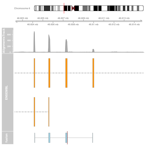
p2 = plotTracks(list(itrack, gtrack, alTrack, biomTrack, brkendTrack),
from = plot.start, to = plot.end,
sizes = c(0.5, 0.5, 1, 3, 0.5))
Plot a circos of all fusions using ggbio
We will plot the full fusion dataset as a circos plot using the ggbio package. A small amount of setup is required.
Reference genome preparation
First obtain the human genome hg19 chromosome lengths from the BSgenome.Hsapiens.UCSC.hg19 package. Create a SeqInfo object for the chromosome sequences of hg19.
library(BSgenome.Hsapiens.UCSC.hg19)

## Loading required package: BSgenome
## Loading required package: Biostrings
## Loading required package: rtracklayer

genome <- Seqinfo(
  seqnames = seqnames(Hsapiens),
  seqlengths = seqlengths(Hsapiens),
  genome = "hg19"
)
We will be working with NCBI 1, 2, 3… named chromosomes rather than chr1, chr2, chr3…
seqlevelsStyle(genome) <- "NCBI"
Subset to the chromosomes we are interested in plotting.
chromosomes = as.character(c(seq(22), "X"))
genome = genome[chromosomes]
We will also require the chromosomes represented as a GRanges object.
genome.ranges = GRanges(
  seqnames = seqnames(genome),
  strand = "*",
  ranges = IRanges(start = 1, width = seqlengths(genome)),
  seqinfo = genome
)
genome.ranges

## GRanges object with 23 ranges and 0 metadata columns:
##        seqnames         ranges strand
##           <Rle>      <IRanges>  <Rle>
##    [1]        1 [1, 249250621]      *
##    [2]        2 [1, 243199373]      *
##    [3]        3 [1, 198022430]      *
##    [4]        4 [1, 191154276]      *
##    [5]        5 [1, 180915260]      *
##    ...      ...            ...    ...
##   [19]       19 [1,  59128983]      *
##   [20]       20 [1,  63025520]      *
##   [21]       21 [1,  48129895]      *
##   [22]       22 [1,  51304566]      *
##   [23]        X [1, 155270560]      *
##   -------
##   seqinfo: 23 sequences from hg19 genome
Plotting chromosomes in a circle
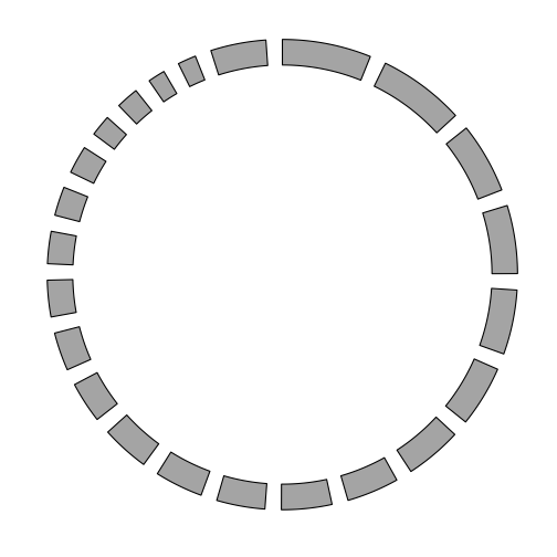
Using the GRanges representation of the chromosome lengths, we can draw a basic plot of the chromosomes in a circle.
p <- ggbio() +
  circle(genome.ranges, geom = "ideo", fill = "gray70")
p
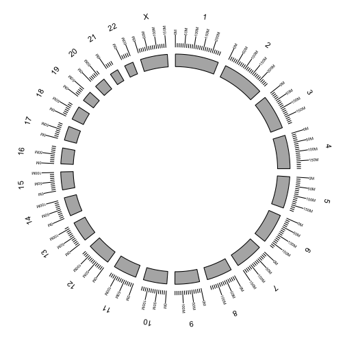
Additional tracks are added using the + operator. Add a scale and chromosome name.
p <- ggbio() +
  circle(genome.ranges, geom = "ideo", fill = "gray70") +
  circle(genome.ranges, geom = "scale", size = 2) +
  circle(genome.ranges, geom = "text", aes(label = seqnames), vjust = -1, size = 4)
p
We are now ready the plot arcs within and between chromosomes representing fusions between genes.
Subset the data by the chromosomes we would like to plot. Also remove low probability events.
data = data[
  data$gene_chromosome1 %in% as.character(chromosomes) &
  data$gene_chromosome2 %in% as.character(chromosomes) &
  data$probability > 0.75,]
Creating a GRanges object for your fusions
Create a GRanges object for the fusions. To do this, we must first create a GRanges object for all the fusion ends together, then split that object into a GrangesList with two elements, one for fusion end 1 and another for fusion end 2. Finally, we add fusion end 2 to the meta data of fusion end 1.
First step, create a GRanges object of all the data, using the c() function to concatenate chromosome, strand and position. Add the mate metadata field to represent the end of the fusion for each entry in the GRanges object.
Important: you must provide a
SeqInfoobject asggbiorequires information about the chromosome lengths
fusion_ends = GRanges(
  seqnames = c(data$gene_chromosome1, data$gene_chromosome2),
  strand = c(data$genomic_strand1, data$genomic_strand2),
  ranges = IRanges(start=c(data$genomic_break_pos1, data$genomic_break_pos2), width=1),
  seqinfo = genome,
  mate = c(rep(0, length(data$gene_chromosome1)), rep(1, length(data$gene_chromosome2))))
Second step, split the GRanges object on the mate field to create a GRangesList with two elements, one containing the fusion ends in gene 1 and the other the fusion ends in gene 2.
fusion_ends_list <- split(fusion_ends, values(fusion_ends)$mate)
Third step, create a fusions GRanges object that is the gene 1 fusion ends linked to the gene 2 fusion ends. Create the fusions object for the first end, then add the second end as the fusedto metadata field.
fusions = fusion_ends_list[[1]]
fusions$fusedto = fusion_ends_list[[2]]
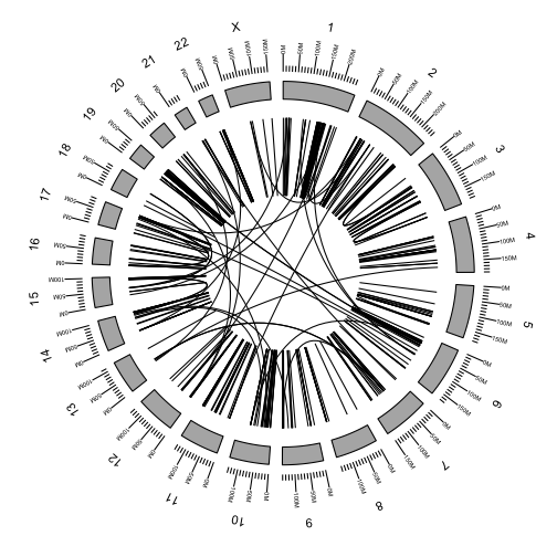
Plotting links
Add the rearrangements to the plot using the link geom argument.
p <- ggbio() +
  circle(fusions, geom = "link", linked.to = "fusedto") +
  circle(genome.ranges, geom = "ideo", fill = "gray70") +
  circle(genome.ranges, geom = "scale", size = 2) +
  circle(genome.ranges, geom = "text", aes(label = seqnames), vjust = -1, size = 4)
p
We can color the links by any of the fusion attributes in the table.
colnames(data)

##  [1] "cluster_id"                     "splitr_sequence"
##  [3] "splitr_count"                   "splitr_span_pvalue"
##  [5] "splitr_pos_pvalue"              "splitr_min_pvalue"
##  [7] "adjacent"                       "altsplice"
##  [9] "break_adj_entropy1"             "break_adj_entropy2"
## [11] "break_adj_entropy_min"          "breakpoint_homology"
## [13] "breakseqs_estislands_percident" "cdna_breakseqs_percident"
## [15] "deletion"                       "est_breakseqs_percident"
## [17] "eversion"                       "exonboundaries"
## [19] "expression1"                    "expression2"
## [21] "gene1"                          "gene2"
## [23] "gene_align_strand1"             "gene_align_strand2"
## [25] "gene_chromosome1"               "gene_chromosome2"
## [27] "gene_end1"                      "gene_end2"
## [29] "gene_location1"                 "gene_location2"
## [31] "gene_name1"                     "gene_name2"
## [33] "gene_start1"                    "gene_start2"
## [35] "gene_strand1"                   "gene_strand2"
## [37] "genome_breakseqs_percident"     "genomic_break_pos1"
## [39] "genomic_break_pos2"             "genomic_ends1"
## [41] "genomic_ends2"                  "genomic_starts1"
## [43] "genomic_starts2"                "genomic_strand1"
## [45] "genomic_strand2"                "interchromosomal"
## [47] "interrupted_index1"             "interrupted_index2"
## [49] "inversion"                      "library_name"
## [51] "max_map_count"                  "max_repeat_proportion"
## [53] "mean_map_count"                 "min_map_count"
## [55] "num_multi_map"                  "num_splice_variants"
## [57] "orf"                            "read_through"
## [59] "repeat_proportion1"             "repeat_proportion2"
## [61] "span_count"                     "span_coverage1"
## [63] "span_coverage2"                 "span_coverage_max"
## [65] "span_coverage_min"              "splice_score"
## [67] "splicing_index1"                "splicing_index2"
## [69] "transcript1"                    "transcript2"
## [71] "probability"
First add the orf attribute to the metadata of our GRanges object.
fusions$orf = data$orf
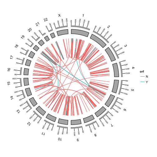
Use aes to color the fusions by whether or not they preserve the open reading frame of the fusion.
p <- ggbio() +
  circle(fusions, geom = "link", linked.to = "fusedto", aes(color = orf)) +
  circle(genome.ranges, geom = "ideo", fill = "gray70") +
  circle(genome.ranges, geom = "scale", size = 2) +
  circle(genome.ranges, geom = "text", aes(label = seqnames), vjust = -1, size = 4)
p