Overview
The goal of this practical session is to identify structural variants (SVs) in a human genome by identifying both discordant paired-end alignments and split-read alignments that. If you recall from the lecture, discordant paired-end alignments conflict with the alignment patterns that we expect (i.e., concordant alignments) for the DNA library and sequencing technology we have used. For example, given a ~500bp paired-end Illumina library, we expect pairs to align in F/R orientation and we expect the ends of the pair to align roughly 500bp apart. Pairs that align too far apart suggest a potential deletion in the DNA sample’s genome. As you may have guessed, the trick is how we define what “too far” is — this depends on the fragment size distribution of the data. Split-read alignments contain SV breakpoints and consequently, then DNA sequences up- and down-stream of the breakpoint align to disjoint locations in the reference genome.
In this session, we will use LUMPY, a SV detection tool developed jointly by the lab of Aaron Quinlan and Ira Hall. LUMPY combines alignment signals from both discordant paired-end and split-read alignments to identify SV breakpoints. If you are interested in LUMPY, you can read the full manuscript here.
The dataset we are using comes from the Illumina Platinum Genomes (http://www.illumina.com/platinumgenomes/) Project, which is a 50X-coverage dataset of the NA12891/NA12892/NA12878 trio. The raw data can be downloaded from the following URL: http://www.ebi.ac.uk/ena/data/view/ERP001960.
Our focus will be on chromosome 20, as processing three whole human genomes worth of data is intractable given the time allowed for this session.
Preliminaries
Amazon node
Read these directions for information on how to log in to your assigned Amazon node.
Work directory
Let’s create a new work directory for this module within our workspace:
rm -rf ~/workspace/module6
mkdir -p ~/workspace/module6
cd ~/workspace/module6
Create symbolic links to all of the files that are relevant to the SV discovery exercise.
ln -s ~/CourseData/HT_data/Module6/* .
Note:
The ln -s command adds symbolic links of all of the files contained in the (read-only) ~/CourseData/HT_data/Module6 directory.
In this step, we created a new directory that will store all of the files created in this lab. The ln -s command adds symbolic links of all of the files contained in the ~/CourseData sub-directories that are relevant to the SV module. This directory contains all of the alignment files (in BAM format, as you will recall) and genome annotations that we’ll need during the lab.
At this point you should have the following files:
ubuntu@ip-10-164-192-186:~/workspace/module6$ ls
bam  delly_call  fastq  pairend_distro.py  reference  RunModule6.sh
Looking in the bam directory, you should see:
ubuntu@ip-10-164-192-186:~/workspace/module6$ ls bam
backup                                    NA12878_S1.chr20.20X.pairs.posSorted.bam.bai
discordants                               NA12891_S1.chr20.20X.pairs.posSorted.bam
NA12878.molelculo.chr20.bam               NA12891_S1.chr20.20X.pairs.posSorted.bam.bai
NA12878.molelculo.chr20.bam.bai           NA12892_S1.chr20.20X.pairs.posSorted.bam
NA12878.pacbio.chr20.bam                  NA12892_S1.chr20.20X.pairs.posSorted.bam.bai
NA12878.pacbio.chr20.bam.bai              README.md
NA12878_S1.chr20.20X.pairs.posSorted.bam  validated
Align DNA with BWA-MEM
This step has been done for you in the interest of time, but the commands are shown so that you can reproduce the results later. The advantage of using BWA-MEM in the context of SV discovery is that it produces both paired-end and split-read alignments in a single BAM output file. In contrast, prior to BWA-MEM, one typically had to use two different aligners in order to produce both high quality paired-end and split-read alignments.
In the alignment commands, note the use of the -M parameter to mark shorter split hits as secondary.
#################
 # Align NA12878 #
 #################
 # bwa mem hg19.fa \
 #         fastq/NA12878_S1.chr20.20X.1.fq \
 #         fastq/NA12878_S1.chr20.20X.2.fq \
 #         -M \
 #   | samtools view -S -b - \
 #   > bam/backup/NA12878_S1.chr20.20X.pairs.readSorted.bam
#################
 # Align NA12891 #
 #################
 # bwa mem hg19.fa \
 #         fastq/NA12891_S1.chr20.20X.1.fq \
 #         fastq/NA12891_S1.chr20.20X.2.fq \
 #         -M \
 #   | samtools view -S -b - \
 #   > bam/backup/NA12891_S1.chr20.20X.pairs.readSorted.bam
#################
 # Align NA12892 #
 #################
 # bwa mem hg19.fa \
 #         fastq/NA12892_S1.chr20.20X.1.fq \
 #         fastq/NA12892_S1.chr20.20X.2.fq \
 #         -M \
 #   | samtools view -S -b - \
 #   > bam/backup/NA12892_S1.chr20.20X.pairs.readSorted.bam
Characterize the fragment size distribution
We have used BWA-MEM to align all of the Illumina paired-end sequences (in FASTQ format) to the human genome. Before we can attempt to identify structural variants via discordant alignments, we must first characterize the fragment size distribution — this describes the size of concordant (i.e., they align in the expected orientation and with the expected distance between the ends) alignments, and the corollary is that we can also use the size distribution to decide the size threshold for discordant alignments. The following script, taken from the distribution of LUMPY extracts F/R pairs from a BAM file and computes the mean and stdev of the F/R alignments. It also generates a density plot of the fragment size distribution.
Calculation of the fragment distribution for NA12878.
samtools view bam/backup/NA12878_S1.chr20.20X.pairs.readSorted.bam \
   | ./pairend_distro.py -r 101 -X 4 -N 10000 \
   -o NA12878_S1.chr20.20X.pairs.histo \
   > NA12878_S1.chr20.20X.pairs.params
Calculation of the fragment distribution for NA12891.
samtools view bam/backup/NA12891_S1.chr20.20X.pairs.readSorted.bam \
   | ./pairend_distro.py -r 101 -X 4 -N 10000 \
   -o NA12891_S1.chr20.20X.pairs.histo \
   > NA12891_S1.chr20.20X.pairs.params
Calculation of the fragment distribution for NA12892.
samtools view bam/backup/NA12892_S1.chr20.20X.pairs.readSorted.bam \
   | ./pairend_distro.py -r 101 -X 4 -N 10000 \
   -o NA12892_S1.chr20.20X.pairs.histo \
   > NA12892_S1.chr20.20X.pairs.params
At this point you should have the following files:
ubuntu@ip-10-164-192-186:~/workspace/module6$ ls
bam         NA12878_S1.chr20.20X.pairs.histo   NA12891_S1.chr20.20X.pairs.params  pairend_distro.py
delly_call  NA12878_S1.chr20.20X.pairs.params  NA12892_S1.chr20.20X.pairs.histo   reference
fastq       NA12891_S1.chr20.20X.pairs.histo   NA12892_S1.chr20.20X.pairs.params  RunModule6.sh
Let’s take a peak at the first few lines of the histogram file that was produced:
head -n 10 NA12878_S1.chr20.20X.pairs.histo
Expected results:
0   0.0
1	0.000200461060439
2	0.000300691590659
3	0.000300691590659
4	0.000200461060439
5	0.000200461060439
6	0.000300691590659
7	0.00010023053022
8	0.00010023053022
9	0.00010023053022
Let’s use R to plot the fragment size distribution. First, launch R from the command line.
R
Now, within R, execute the following commands:
size_dist <- read.table('NA12878_S1.chr20.20X.pairs.histo')
 pdf(file = "NA12878.fragment.hist.pdf")
 plot(size_dist[,1], size_dist[,2], type='h')
 dev.off()
 size_dist <- read.table('NA12891_S1.chr20.20X.pairs.histo')
 pdf(file = "NA12891.fragment.hist.pdf")
 plot(size_dist[,1], size_dist[,2], type='h')
 dev.off()
 size_dist <- read.table('NA12892_S1.chr20.20X.pairs.histo')
 pdf(file = "NA12892.fragment.hist.pdf")
 plot(size_dist[,1], size_dist[,2], type='h')
 dev.off()
 quit("no")
At this point, you should have the following files:
ubuntu@ip-10-164-192-186:~/workspace/module6$ ls
bam                               NA12878_S1.chr20.20X.pairs.params  NA12892_S1.chr20.20X.pairs.histo
delly_call                        NA12891.fragment.hist.pdf          NA12892_S1.chr20.20X.pairs.params
fastq                             NA12891_S1.chr20.20X.pairs.histo   pairend_distro.py
NA12878.fragment.hist.pdf         NA12891_S1.chr20.20X.pairs.params  reference
NA12878_S1.chr20.20X.pairs.histo  NA12892.fragment.hist.pdf          RunModule6.sh
If successful, you should be able to access the 3 PDF files at the following URLs:
 http://cbwXX.dyndns.info/module6/NA12878.fragment.hist.pdf
 http://cbwXX.dyndns.info/module6/NA12891.fragment.hist.pdf
 http://cbwXX.dyndns.info/module6/NA12892.fragment.hist.pdf
Note: Copy and paste the URL below into your browser, but change the “XX” in the URL to your student number.
Spend some time thinking about what this plot means for identifying discordant alignments.
What does the mean fragment size appear to be?
Are all 3 graphs the same?
Is that good or bad?
Extract discordant alignments
This step has been done for you in the interest of time, but the commands are shown so that you can reproduce the results later.Now that we understand the shape of each sample’s fragment size distribution, we can extract the subset of discordant alignments from the BAM in order to create a much smaller BAM file for LUMPY.
Exlude:
 exclude properly-paired pairs (0x0002)
 exclude not-primary alignments (0x0100)
 exclude unmapped (0x0004)
 exclude mate unmapped (0x0008)
 exclude duplicates (0x0400)
Steps:
 ################################################
 # Extract discordant PE alignments for NA12878 #
 ################################################
 # samtools view -u -F 0x0002 bam/backup/NA12878_S1.chr20.20X.pairs.readSorted.bam  \
 #    |  samtools view -u -F 0x0100 - \
 #    | samtools view -u -F 0x0004 - \
 #    | samtools view -u -F 0x0008 - \
 #    | samtools view -b -F 0x0400 - \
 #    > NA12878_S1.chr20.20X.pairs.disc.readSorted.bam

 ################################################
 # Extract discordant PE alignments for NA12891 #
 ################################################
 # samtools view -u -F 0x0002 bam/backup/NA12891_S1.chr20.20X.pairs.readSorted.bam  \
 #    |  samtools view -u -F 0x0100 - \
 #    | samtools view -u -F 0x0004 - \
 #    | samtools view -u -F 0x0008 - \
 #    | samtools view -b -F 0x0400 - \
 #    > NA12891_S1.chr20.20X.pairs.disc.readSorted.bam

 ################################################
 # Extract discordant PE alignments for NA12892 #
 ################################################
 # samtools view -u -F 0x0002 bam/backup/NA12891_S1.chr20.20X.pairs.readSorted.bam  \
 #    |  samtools view -u -F 0x0100 - \
 #    | samtools view -u -F 0x0004 - \
 #    | samtools view -u -F 0x0008 - \
 #    | samtools view -b -F 0x0400 - \
 #    > NA12891_S1.chr20.20X.pairs.disc.readSorted.bam
Now we must sort the discordant alignments by chromosome coordinates so that LUMPY can detect SVs.
 ################################################
 # Sort discordant PE alignments for NA12878 #
 ################################################
 # samtools sort NA12878_S1.chr20.20X.pairs.disc.readSorted.bam NA12878_S1.chr20.20X.pairs.disc.posSorted

 ################################################
 # Sort discordant PE alignments for NA12891 #
 ################################################
 # samtools sort NA12891_S1.chr20.20X.pairs.disc.readSorted.bam NA12891_S1.chr20.20X.pairs.disc.posSorted

 ################################################
 # Sort discordant PE alignments for NA12892 #
 ################################################
 # samtools sort NA12892_S1.chr20.20X.pairs.disc.readSorted.bam NA12892_S1.chr20.20X.pairs.disc.posSorted
Extract “split” alignments
This step has been done for you in the interest of time, but the commands are shown so that you can reproduce the results later.Similarly, we must create a BAM file for LUMPY that contains the subset of split-read alignments. This step depends upon a script that is provided in the LUMPY software package.
 ################################################
 # Extract split alignments for NA12878         #
 ################################################
 samtools view -h NA12878_S1.chr20.20X.pairs.disc.readSorted.bam \
   | scripts/extractSplitReads_BwaMem -i stdin \
   | samtools view -Sb - \
   > NA12878_S1.chr20.20X.yaha.pairs.readSorted.bam

 ################################################
 # Extract split alignments for NA12891         #
 ################################################
 samtools view -h NA12891_S1.chr20.20X.pairs.disc.readSorted.bam \
   | scripts/extractSplitReads_BwaMem -i stdin \
   | samtools view -Sb - \
   > NA12891_S1.chr20.20X.yaha.pairs.readSorted.bam

 ################################################
 # Extract split alignments for NA12892         #
 ################################################
 samtools view -h NA12892_S1.chr20.20X.pairs.disc.readSorted.bam \
   | scripts/extractSplitReads_BwaMem -i stdin \
   | samtools view -Sb - \
   > NA12892_S1.chr20.20X.yaha.pairs.readSorted.bam
Now we must sort the split alignments by chromosome coordinates so that LUMPY can detect SVs.
 ################################################
 # Sort discordant PE alignments for NA12878 #
 ################################################
 # samtools sort NA12878_S1.chr20.20X.yaha.pairs.readSorted.bam NA12878_S1.chr20.20X.yaha.pairs.posSorted

 ################################################
 # Sort discordant PE alignments for NA12891 #
 ################################################
 # samtools sort NA12891_S1.chr20.20X.yaha.pairs.readSorted.bam NA12891_S1.chr20.20X.yaha.pairs.posSorted

 ################################################
 # Sort discordant PE alignments for NA12892 #
 ################################################
 # samtools sort NA12892_S1.chr20.20X.yaha.pairs.readSorted.bam NA12892_S1.chr20.20X.yaha.pairs.posSorted
Run LUMPY to detect SVs!
Finnaly, we can now run LUMPY to detect SVs! Recall from the SV lecture that LUMPY’s key strength is that it combines multiple alignment signals (e.g. paired-end and split-read) into a single probabilistic framework for SV detection. This is why we have (ahead of time) created BAM files reflecting the discordant and split-read alignments for each individual in the trio.
Before we run LUMPY, let’s explain some of the parameters:
Each piece of evidence has a weight, and each possible call has an evidence set. The sum of weights in the evidence set must be above this value.
-mw minimum weight for a call
Each predicted breakpoint interval has a probability array associated with it. The intervals can be trimmed of values that are below some trimming percentile. NOTE: We recommend “-tt 0.0” (no trimming) since LUMPY now reports both the 95% confidence interval and the most probable single base for each breakpoint.
-tt trim threshold
Now, let’s run LUMPY:
 lumpy \
   -mw 4 \
   -tt 0 \
   -pe bam_file:bam/discordants/NA12878_S1.chr20.20X.pairs.disc.posSorted.bam,histo_file:NA12878_S1.chr20.20X.pairs.histo,mean:325.744225577444,stdev:72.5462416180379,read_length:100,min_non_overlap:100,discordant_z:4,back_distance:20,weight:1,id:781,min_mapping_threshold:10 \
   -sr bam_file:bam/discordants/NA12878_S1.chr20.20X.yaha.pairs.posSorted.bam,back_distance:20,min_mapping_threshold:100,weight:1,id:782,min_clip:20 \
   -pe bam_file:bam/discordants/NA12891_S1.chr20.20X.pairs.disc.posSorted.bam,histo_file:NA12891_S1.chr20.20X.pairs.histo,mean:306.423157684233,stdev:63.2546229114364,read_length:100,min_non_overlap:100,discordant_z:4,back_distance:20,weight:1,id:911,min_mapping_threshold:10 \
   -sr bam_file:bam/discordants/NA12891_S1.chr20.20X.yaha.pairs.posSorted.bam,back_distance:20,min_mapping_threshold:100,weight:1,id:912,min_clip:20 \
   -pe bam_file:bam/discordants/NA12892_S1.chr20.20X.pairs.disc.posSorted.bam,histo_file:NA12892_S1.chr20.20X.pairs.histo,mean:310.187881211877,stdev:65.432044115405,read_length:100,min_non_overlap:100,discordant_z:4,back_distance:20,weight:1,id:921,min_mapping_threshold:10 \
   -sr bam_file:bam/discordants/NA12892_S1.chr20.20X.yaha.pairs.posSorted.bam,back_distance:20,min_mapping_threshold:100,weight:1,id:922,min_clip:20 \
   > lumpy.trio.bedpe 2> lumpy.trio.err
If successful, you should see the output below when you run the following command:
less -S lumpy.trio.bedpe
Expected output:
 chr20 60570619  60570658  chr20 60570924  60570964  119 1.53873e-24 + - TYPE:DELETION IDS:781,1;782,1;911,1;912,1;921,6 STRANDS:+-,10 MAX:chr20:60570638;chr20:60570964 95:chr20:60570635-60570641;chr20:60570964-60570964
 chr20 61304231  61304269  chr20 61305118  61305152  120 1.39004e-58 + - TYPE:DELETION IDS:781,8;911,7;912,2;921,8;922,1 STRANDS:+-,26 MAX:chr20:61304250;chr20:61305152 95:chr20:61304248-61304252;chr20:61305152-61305152
 chr20 61544634  61544658  chr20 61544653  61544678  121 3.66156e-06 + - TYPE:DELETION IDS:782,2;922,4 STRANDS:+-,6  MAX:chr20:61544647;chr20:61544666 95:chr20:61544646-61544648;chr20:61544665-61544667
 chr20 61724682  61724825  chr20 61725464  61725611  122 0.00316456  + - TYPE:DELETION IDS:781,19;911,13;921,6 STRANDS:+-,38 MAX:chr20:61724703;chr20:61725593 95:chr20:61724697-61724728;chr20:61725567-61725596
 chr20 62123284  62123532  chr20 62123881  62124304  123 5.32664e-15 - + TYPE:DUPLICATION  IDS:781,2;911,2;921,1 STRANDS:-+,5  MAX:chr20:62123512;chr20:62123902 95:chr20:62123404-62123515;chr20:62123899-62124046
 chr20 62267516  62267812  chr20 62267925  62268064  124 0.00333333  + - TYPE:DELETION IDS:781,9;911,11  STRANDS:+-,20 MAX:chr20:62267537;chr20:62268043 95:chr20:62267532-62267583;chr20:62267986-62268048
 chr20 62596211  62596418  chr20 62597342  62597467  125 3.40999e-39 + - TYPE:DELETION IDS:781,6;911,4;921,5 STRANDS:+-,15 MAX:chr20:62596232;chr20:62597467 95:chr20:62596226-62596273;chr20:62597467-62597467
 chr20 62709518  62709540  chr20 62709622  62709645  126 1.48224e-06 - + TYPE:DUPLICATION  IDS:912,2;922,5 STRANDS:-+,7  MAX:chr20:62709530;chr20:62709634 95:chr20:62709529-62709531;chr20:62709633-62709635
 chr20 62719940  62719951  chr20 62720272  62720304  127 0.027027  - + TYPE:DUPLICATION  IDS:781,6;782,2;911,5;921,10  STRANDS:-+,23 MAX:chr20:62719949;chr20:62720304 95:chr20:62719942-62719952;chr20:62720304-62720304
 chr20 62899477  62899514  chr20 62903537  62903575  128 0.000127914 + - TYPE:DELETION IDS:782,3;912,1 STRANDS:+-,4  MAX:chr20:62899497;chr20:62903557 95:chr20:62899496-62899498;chr20:62903556-62903558
Setting up IGV for SV visualization
Load the following BED file of validated (more on this later) LUMPY SV calls. First, we need to rename the file for IGV. Let’s focus on validated SVs that are >= 500 base pairs.
 cat bam/validated/lumpy.78.91.92.bedpe.slop0.val \
 | awk '$(NF-1)>1 || $NF>0' \
 | awk '{print $1"\t"$2"\t"$6"\t"$11}' \
 | awk '{if (($3-$2) >= 500) {print}}' \
 > lumpy.validated.svs.bed
Look at some of the structural variant calls in the .bed file.
less -S lumpy.validated.svs.bed
At this point, you should have the following files:
ubuntu@ip-10-182-231-187:~/workspace/module6$ ls
bam                        NA12878_S1.chr20.20X.pairs.histo   NA12892_S1.chr20.20X.pairs.histo
fastq                      NA12878_S1.chr20.20X.pairs.params  NA12892_S1.chr20.20X.pairs.params
**lumpy.trio.bedpe**           NA12891.fragment.hist.pdf          pairend_distro.py
**lumpy.trio.err**             NA12891_S1.chr20.20X.pairs.histo   RunModule6.sh
**lumpy.validated.svs.bed**    NA12891_S1.chr20.20X.pairs.params
NA12878.fragment.hist.pdf  NA12892.fragment.hist.pdf
Load the following validated BED file in to IGV. These are the original BAM alignment files for the trio. Use “File->Load From URL”:
[http://cbwXX.dyndns.info/module6/lumpy.validated.svs.bed](http://cbwXX.dyndns.info/module6/lumpy.validated.svs.bed)
Navigate to the following location:
chr20:31,310,769-31,312,959
You should see something like the following (FIGURE):
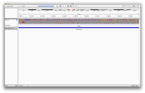 ”
”
Load the following BAM files in to IGV. These are the original BAM alignment files for the trio. Use “File->Load From URL”:
 [http://cbwXX.dyndns.info/module6/bam/NA12878_S1.chr20.20X.pairs.posSorted.bam](http://cbwXX.dyndns.info/module6/bam/NA12878_S1.chr20.20X.pairs.posSorted.bam)
 [http://cbwXX.dyndns.info/module6/bam/NA12891_S1.chr20.20X.pairs.posSorted.bam](http://cbwXX.dyndns.info/module6/bam/NA12891_S1.chr20.20X.pairs.posSorted.bam)
 [http://cbwXX.dyndns.info/module6/bam/NA12892_S1.chr20.20X.pairs.posSorted.bam](http://cbwXX.dyndns.info/module6/bam/NA12892_S1.chr20.20X.pairs.posSorted.bam)
You should see something like the following (FIGURE):
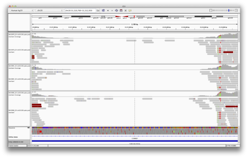 ”
”
The above SVs were “validated” by comparing the SVs predicted by LUMPY with sequencing data from the PacBio and Illumina Moleculo technologies. The idea is that these are distinct sequencing technologies (strategies) with their own error modalities. If we see evidence for SVs from these technologies at the same loci as predicted by LUMPY, it is very unlikely that they are false SV predictions. Let’s load the Moleculo alignments for NA12878.
[http://cbwXX.dyndns.info/module6/bam/NA12878.molelculo.chr20.bam](http://cbwXX.dyndns.info/module6/bam/NA12878.molelculo.chr20.bam)
You should see something like the following (FIGURE):
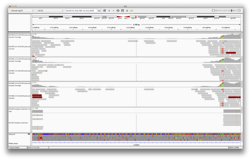 ”
”
Now, we need to configure IGV such that we can more clearly see the alignments that support the SV prediction. First we must make sure that the alignments are colored by insert size and orientation. For each of the BAM tracks, right-click on the track and select the following:
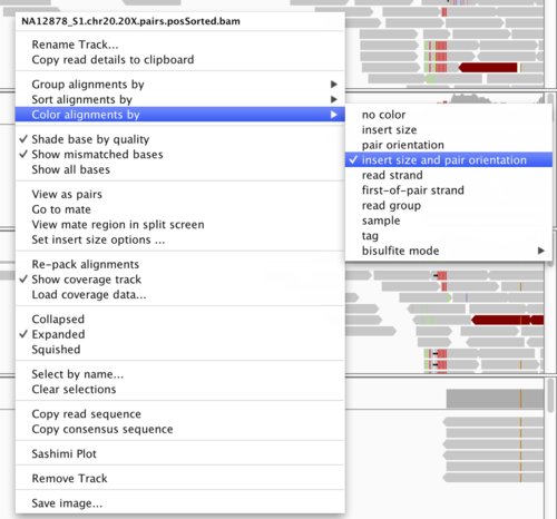 ”
”
Next, we want to set the size range of the expected “concordant” alignments. Repeat for each alignment track.
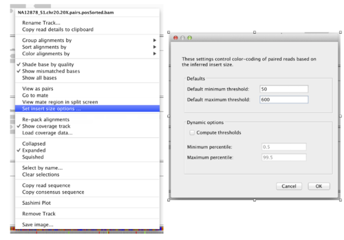 ”
”
Explore the SVs
*Is the variant at chr20:31,310,769-31,312,959 found in each member of the trio? What are the genotypes for each member of the trio at this locus (e.g., hemizygous, homozygous)?* *What about the variant at chr20:37,054,372-37,056,562? Does the evidence in the Moleculo track mimic the evidence in the Illumina track for NA12878?* *What about chr20:42,269,896-42,278,072?*Continue exploring the data!
For example, navigate to other SV loci by clicking on the “lumpy.validated.svs.bed” track and using “Ctrl+F” and “Ctrl+B”.
Overall script
**NOTE:**If you ever become truly lost in this lab, you can use the lab script to automatically perform all of the steps listed here. If you are logged into your CBW account, just run: ~/CourseData/HT_data/Module6/RunModule6.sh. You can also download the file if you want to bring it home with you.
Acknowledgements
This module is heavily based on a previous module prepared by Aaron Quinlan.