Introduction
Description of the lab
Welcome to the lab for Genome Visualization! This lab will introduce you to the Savant Genome Browser, one of the most popular visualization tools for High Throughput Sequencing (HTS) data.
After this lab, you will be able to:
- download, format, and visualize a variety of genomic data
- very quickly navigate around the genome
- visualize HTS read alignments
- validate SNP calls by eye
- validate CNV calls by eye
Things to know before you start:
- The lab may take between 1-2 hours, depending on your familiarity with genome browsing. At the beginning of each section is an approximate amount of time that you might spend on it. Don’t worry if you don’t complete the lab! It will be made available for you to complete later.
- There are a few thought-provoking Questions pertaining to sections of the lab. These are optional, and may take more time, but are meant to help you better understand the visualizations you are seeing. These questions will be denoted by boxes, as follows:
Question(s):
* Thought-provoking question goes here
Requirements
- Savant Genome Browser
- Ability to run Java
Compatibility
This tutorial was intended for Savant v2.0.3, which is available on our Download page. It is strongly recommended that you use this version, as other versions may not be compatible. If you have installed a former version, please uninstall it before and install the latest version.
Troubleshooting
If you are performing this lab during the workshop, feel free to ask for help from the TAs or Instructors. Otherwise, the Savant Team would be glad to help via email to support@genomesavant.com.
Check the online wiki
Your instructors may update the lab with clarifications or more bonus sections.
Visualization Part 1: Getting familiar with the Savant Genome Browser
Samtools is useful for processing the raw data, but there are better tools available to visualize the mappings. We will be visualizing the alignments using the Savant Genome Browser, a popular visualization tool for HTS data. Unlike IGV, another popular tool you’ve already used, Savant lets us visualize the matepair information in a way that is important for your understanding of structural variations. First, lets familiarize ourselves with it.
Get familiar with the interface
Load a Genome
Savant requires that a genome be loaded before tracks. For this lab, we will be loading the human genome as follows:
- Click File > Load a Genome.
- Select URL
- Paste in the URL of the genome from one of the following mirrors:
- main mirror: http://your_instance_url.com/module3/fa/hg19.fa.savant
- mirror 1: http://compbio.cs.toronto.edu/savant/data/dropbox/icgc/hg19.fa.savant
- mirror 2: http://compbio.cs.toronto.edu/savant/data/dropbox2/hg19.fa.savant
- mirror 3: http://genomesavant.com/savant/data/hg19/hg19.fa.savant
Navigation
Savant will load the hg19 sequence and a gene track. The tracks are stacked on top of each other. You can likely identify which track is which by consulting the track path printed on the Title Bar of each track. You’ll notice that the sequence track is completely gray, since this assembly has been padded at the beginning with 10,000 N’s. Navigate to chr1:10,000-11,000 by entering this into the location field (in the top-left corner of the interface) and clicking Go.
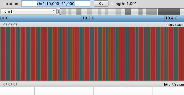
Savant displays the sequence of letters in a genome as a sequence of colours (e.g. A = blue). This makes repetitive sequences, like the ones found at the start of this region, easy to identify.
Navigation is possible in Savant in many ways:
If you’re interested you can read about Savant Navigation Shortcuts and Savant Interface Customization. Otherwise, let’s continue to the next section.
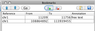
Bookmarking
The Bookmarking module is located on the right side of the interface. Unhide it by right-clicking on the Bookmarks tab and unchecking “Auto Hide”. While you browse around the genome, add some bookmarks by pressing Ctrl/Cmd+B or by clicking the Add Bookmark Icon located on the top of the Bookmarks module.
Loading Read Alignments
Note: Due to server high server load during the workshop, we may need to split the load by hosting the data on a number of different servers. We may assign you different URLs that points to a file containing read alignments to hg19. Please inform the instructor if you are experiencing difficulties loading and navigating these tracks.
Here is a URL that points to chromosome 1 read alignments for an individual from the Thousand Genomes Project:
NA12878 Alignments to hg19:
- main mirror: http://your_instance_url.com/module3/bam/NA12878_chr1.bam
- mirror 1: http://compbio.cs.toronto.edu/savant/data/dropbox/icgc/NA12878_chr1.bam
- mirror 2: http://compbio.cs.toronto.edu/savant/data/dropbox2/NA12878_chr1.bam
- mirror 3: http://compbio.cs.toronto.edu/savant/data/medsavant/serve/tracks/NA12878_chr1.bam
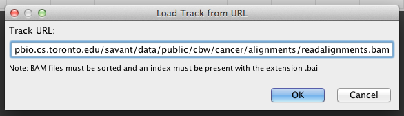
In Savant, choose File > Load Track from URL, enter the URL and click Go.
Visualizing read alignments
The default visualization mode for read alignment tracks when a reference genome is loaded is called Mismatch Mode. In Mismatch Mode, reads are coloured according to the strand to which they map: reads that map to the positive strand are dark blue; those that map to the negative strand are light blue. Where the read sequence mismatches the reference, a coloured box is drawn; the colour of the box represents the letter that exists in the read (using the same colour legend used for displaying the reference).
You can switch visualization modes in two ways:
- Choose a new mode from the Display Mode dropdown of the selected track
- Pressing Ctrl/Cmd+M on the keyboard
The visualization modes for BAM tracks are as follows:
- Standard: show reads without mismatches
- Mismatch: show reads and mismatches
- Read sequence: colour each letter in read sequence
- Read pair (aka Arc): connect read pairs with an arc; the height and width of the arc corresponds to mapped distance
- Mapping Quality mode: make reads transparent according to mapping quality
- Base Quality mode: make positions in reads transparent according to base quality
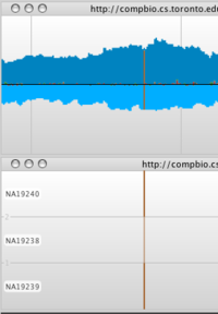
- SNP: show a coverage plot, and the proportion of reads that are mismatched
- Strand SNP: SNP mode, with coverage plots for forward and negative strands separately
Experiment with the various visualization modes and think about which would be best for specific tasks (e.g. quality control, SNP calling, CNV finding)
Visualization Part 2: Inspecting SNPs
For this part, we continue using NA12878 alignments to hg19. You can find the path to the BAM file listed above.
In Savant, choose File > Load Track from URL, enter the abovelisted URL and click Go.
Next, we are going to load variants that have been identified in this individual. These variants are in VCF format but have been previously formatted for use with Savant. NB: Savant will automatically format any VCF file that you load.
Variants from NA12878:
- main mirror: http://your_instance_url.com/module3/vcf/vcfBeta-NA12878-200-37-ASM.vcf.gz
- mirror 1: http://compbio.cs.toronto.edu/savant/data/dropbox/icgc/vcfBeta-NA12878-200-37-ASM.vcf.gz
- mirror 2: http://compbio.cs.toronto.edu/savant/data/dropbox2/vcfBeta-NA12878-200-37-ASM.vcf.gz
- mirror 3: http://compbio.cs.toronto.edu/savant/data/medsavant/serve/tracks/vcfBeta-NA12878-200-37-ASM.vcf.gz
In Savant, choose File > Load Track from URL, enter the abovelisted URL and click Go.
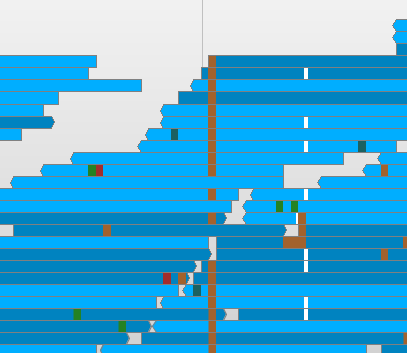
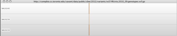
A VCF track will be generated. The track is divided into a number of rows, one row per sample from the VCF file. At positions where variants have been predicted, Savant will color that position according to the predicted call. Heterozygous calls will be semi-transparent, as shown for the second individual in the image below.
Using the Variation Component
The latest version of Savant has a special component for browsing variant files. It is located on the right side, near the bookmarks tab. Click the Variation tab and Toggle auto-hide so that the component is pinned.
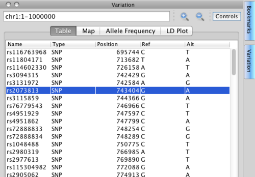
Notice that the Variation component that has a range that is independent of the track range. It always contains the track range, but may be larger, allowing you to view a large number of variants but hone in on them in the tracks.
Make the Variation range chr1:1-1000000. You should see a list of variants like the one in the image above.
This component delivers a number of different views:
- Table: lists all variants within the Variation range
- Map: lists all variants within the Variation range, by individual. The order of individuals from left to right corresponds with their order in the track from top to bottom.
- Allele Frequency: The frequency of each variant in Variation range among the loaded individuals
- LD Plot: measures of linkage between variants in the Variation range
Double-click on a row in the Table view of the Variation component. Savant will center on that variant’s position. Validate with the alignments track if the call looks correct.
Explore the SNP regions, using the Variation component as a guide.
Question(s):
* What level of support seems to be required to call a SNP?
* Why do **less** than half of the reads (usually) support the alternate base in locations of a heterozygous SNP?
* What proportion of the SNPs called do you think are real?
Visualization Part 3: Inspecting Structural Variations
For this part, you’ll need to continue looking at hg19, and the NA12878 alignments to this reference. Links to the .BAM file containing these alignments is listed here.
To ease the load on the servers, load hg19 genome from URL:
- main mirror: http://your_instance_url.com/module3/fa/hg19.fa.savant
- mirror 1: http://compbio.cs.toronto.edu/savant/data/dropbox/icgc/hg19.fa.savant
- mirror 2: http://compbio.cs.toronto.edu/savant/data/dropbox2/hg19.fa.savant
- mirror 3: http://genomesavant.com/savant/data/hg19/hg19.fa.savant
Here is a URL that points to chromosome 1 read alignments for an individual from the Thousand Genomes Project:
NA12878 Alignments to hg19:
- main mirror: http://your_instance_url.com/module3/bam/NA12878_chr1.bam
- mirror 1: http://compbio.cs.toronto.edu/savant/data/dropbox/icgc/NA12878_chr1.bam
- mirror 2: http://compbio.cs.toronto.edu/savant/data/dropbox2/NA12878_chr1.bam
- mirror 3: http://compbio.cs.toronto.edu/savant/data/medsavant/serve/tracks/NA12878_chr1.bam
We will now inspect Structural Variant calls that have been made for this individual. To help you, you will now load a set of bookmarks for these regions. Download http://your_instance_url.com/module3/text/bookmarks.txt or http://compbio.cs.toronto.edu/savant/data/dropbox2/bookmarks.txt to your computer by right-clicking and choosing save. Load this file into the Bookmarks panel by clicking the Folder icon and choosing the file you just downloaded. If prompted to remove existing bookmarks, choose Yes.

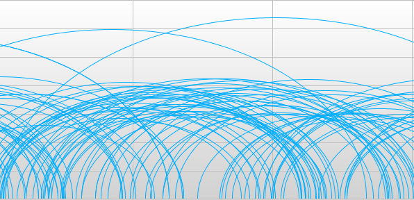
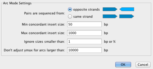
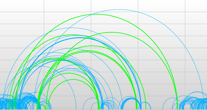
Switch the display mode of the read alignment track by first clicking it, then choosing Display Mode > Read Pair (Arc) mode. In Arc mode the locations of read pair mappings are connected by an arc. Both the height and the width of this arc is proportional to the mapped distance of this pair. This makes discordant read pairs very easy to identify. If you use, Standard mode, structural variations will be very difficult to detect. You can also tell Savant to color discordant read pairs. Click Tools > Filter and enter reasonable settings under Arc Mode Settings. What is “normal” very much depends on the sequencing technology used. For this example, you can enter values shown in the image below and press OK.
Discordant pairs are joined with a purple arc. How are discordant read pairs visualized now?
Now explore the variant regions, using the bookmarks list as a guide.
Normal regions will have mostly concordant matepairs, with distance around 250 and orientation pointed inward. How can you tell which regions are normal?
Large arcs represent pairs which map too far apart compared to the insert size. Small arcs represent pairs that map too closely. Non-blue arcs represent pairs which are mapped in a different orientation than how they were sequenced. ‘Which regions look suspect?
Question(s):
* Try hypothesizing what the sequenced individual's genome looks like. Do the patterns of read pair mappings agree with your hypothesis?
* Can you distinguish between various kinds of structural variations (e.g. **deletions**, **insertions**, **duplications**)?
* Use matepair information to determine the precise breakpoints of some structural variations
Concluding Remarks
You’re done! We hope that you enjoyed the lab and that you continue to enjoy Savant.
If you have any questions, comments, or feature suggestions, the Savant Development Team would be happy to hear from you! Please contact support@genomesavant.com.