Module 4: Downstream analyses & integrative tools

Important notes:

• Please refer to the following guide for instructions on how to connect to Guillimin and submit jobs: using_the_guillimin_hpc.md
• The instructions in this tutorial will suppose you are in a Linux/Max environment. The equivalent tools in Windows are provided in the Guillimin documentation.
• The user class99 is provided here as an example. You should replace it by the username that was assigned to you at the beginning of the workshop.

Introduction

Description of the lab

In this module’s lab, we will explore some of the tools that were covered in the lecture.

• First, we will learn how to use the IHEC Data Portal’s tools to fetch datasets tracks of interest.
• Second, we will explore ChIP-Seq peak prediction files to attempt discovering motifs using HOMER.
• Third, we will use these datasets with the GREAT GO enrichment tool to do functions prediction.

Local software that we will use

• A web browser
• ssh
• scp or WinSCP to transfer results from HOMER to your computer

Tutorial

Connect to the Guillimin HPC

We will need the HPC for some of the steps, so we’ll open a shell access now. Replace class99 with your login name.

ssh class99@guillimin.clumeq.ca

You will be in your home folder. At this step, before continuing, please make sure that you followed the instructions in the section “The first time you log in” of the Guillimin guide. If you don’t, compute jobs will not execute normally.

Prepare directory for module 4

rm -rf ~/module4
mkdir -p ~/module4
cd ~/module4

1- IHEC Data Portal

Exploring available datasets

• Open a web browser on your computer, and load the URL http://epigenomesportal.ca/ihec .

• In the Overview page, click on the “View all” button.

• You will get a grid with all available datasets for IHEC Core Assays.
  • You can filter out visible datasets in the grid using the filtering options at the bottom of the grid.

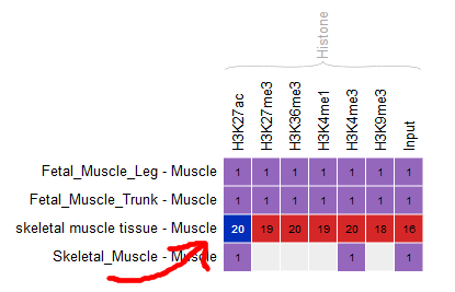
• Go back to the Overview page, and select the following categories of datasets: “Histone” for the “Muscle” cell type.

• Only these categories will now get displayed in the grid. Select the following grid cells:

Visualizing the tracks

• Select “Visualize in Genome Browser”
  • You can see that the datasets are being displayed at a mirror of the UCSC Genome Browser. These are all peaks and signal for the chosen muscle H3K427ac ChIP-Seq datasets. In the Genome Browser, you can expand the tracks by changing visibility from “pack” to “full” and clicking the “Refresh” button.

• You can also download these tracks locally for visualization in IGV. (You can skip this step if you’re comfortable with IGV already)
  • Go back to the IHEC Data Portal tab.
  • Click on the “Download tracks” button at the bottom of the grid.
  • Use the download links to download a few of the tracks.
  • Open them in IGV.

Tracks correlation

You can get a whole genome overview of the similarity of a group of tracks by using the Portal’s correlation tool.

• From the filters at the bottom of the grid, add back datasets for all tissues.

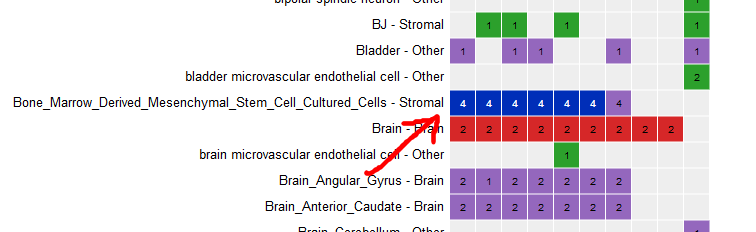
• Select all ChIP-Seq marks for the cell type “Bone Marrow Derived Mesenchymal Stem Cell Cultured Cell”.

• At the bottom of the grid, click on the button “Correlate tracks”.

• You will see that tracks seem to correlate nicely, with activator marks clustering together and repressor marks forming another group. You can zoom out the view at the upper right corner of the popup.

• You can also use the correlation tool to assess whether datasets that are supposed to be similar actually are.

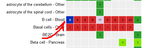
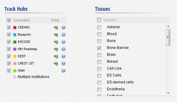
  • Activate the track hubs for all consortia.
  • Click on the grid cell for cell type “B Cell” and assay “H3K27ac”.
  • Click on “Correlate tracks”.
  • One dataset seems to be an outlier… This is either a problem with the quality of the dataset, or the underlying metadata can indicate that something is different (disease status or some other key element).

2- Predicting motifs with HOMER

We will now attempt to detect motifs in peak regions for transcription factor binding sites using HOMER.

• Go back to the default IHEC Data Portal view by clicking “Data Grid” in the top bar.

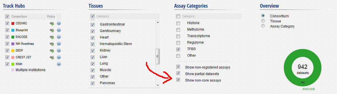
• In the filters at the bottom of the grid, activate non-core IHEC assays, and display only Transcription Factor Binding Sites (TFBS) assays.

• In the grid, select ENCODE datasets for the YY1 assay and the H1hESC cell type.

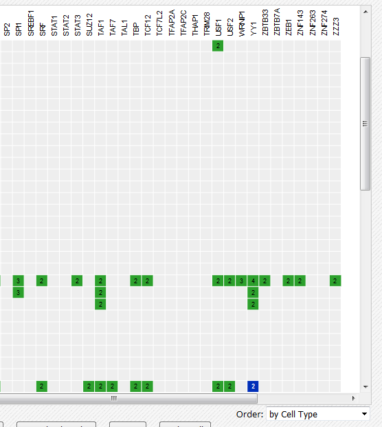
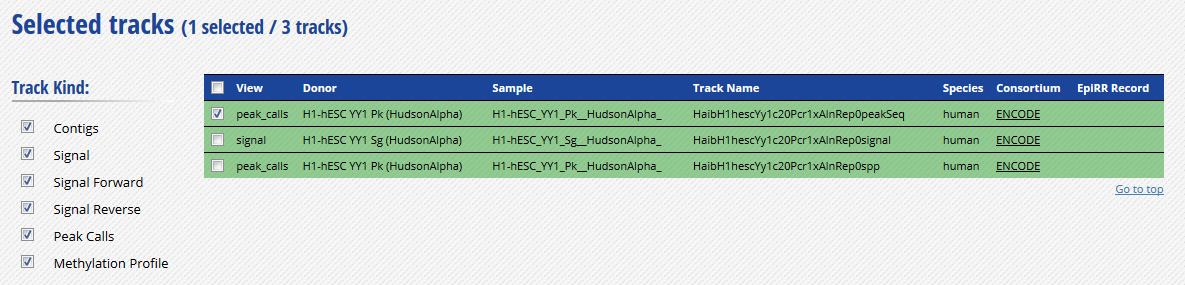
• Go to the track list at the bottom of the grid and select only the peak file “HaibH1hescYy1c20Pcr1xAlnRep0peakSeq”.

• Get the URL to this track by clicking on the “Download datasets” button at the bottom of the grid. The URL should be http://ftp.ebi.ac.uk/pub/databases/ensembl/encode/integration_data_jan2011/byDataType/peaks/jan2011/peakSeq/optimal/hub/peakSeq.optimal.wgEncodeHaibTfbsH1hescYy1c20Pcr1xAlnRep0_vs_wgEncodeHaibTfbsH1hescControlPcr1xAlnRep0.bb.

• Open your Guillimin terminal session, create a directory for our HOMER-related files, and go into it. Then, download the BigBed file.

mkdir homer
cd homer
wget http://ftp.ebi.ac.uk/pub/databases/ensembl/encode/integration_data_jan2011/byDataType/peaks/jan2011/peakSeq/optimal/hub/peakSeq.optimal.wgEncodeHaibTfbsH1hescYy1c20Pcr1xAlnRep0_vs_wgEncodeHaibTfbsH1hescControlPcr1xAlnRep0.bb

• Convert the bigBed file into a bed file using the UCSC set of tools. It is available as a CVMFS module.

module load mugqic/ucsc/20140212
bigBedToBed peakSeq.optimal.wgEncodeHaibTfbsH1hescYy1c20Pcr1xAlnRep0_vs_wgEncodeHaibTfbsH1hescControlPcr1xAlnRep0.bb peakSeq.optimal.wgEncodeHaibTfbsH1hescYy1c20Pcr1xAlnRep0_vs_wgEncodeHaibTfbsH1hescControlPcr1xAlnRep0.bed

• Prepare an output directory for HOMER, and a genome preparsed motifs directory.

mkdir output
mkdir preparsed

• Run the HOMER software to identify motifs in the peak regions. To do so, we will launch a job on the scheduler. Please note that there are two modules necessary here:
  • mugqic/homer/4.7 to run HOMER
  • mugqic/weblogo/2.8.2 to create the nice motifs images that we will visualize in a browser. Don’t load module mugqic/weblogo/3.3, as the input parameters are very different and it will not work with HOMER.

echo 'module load mugqic/homer/4.7 ; module load mugqic/weblogo/2.8.2 ; \
findMotifsGenome.pl peakSeq.optimal.wgEncodeHaibTfbsH1hescYy1c20Pcr1xAlnRep0_vs_wgEncodeHaibTfbsH1hescControlPcr1xAlnRep0.bed \
hg19 output -preparsedDir preparsed -p 2 -S 15' | qsub -l nodes=1:ppn=2 -d .

• HOMER takes a while to execute for a whole genome track like this. Expect this job to take about 30 minutes of runtime, with the current 2 cores setup. In the meantime, we will explore the GO terms enrichment tool GREAT.

3- Looking for GO terms enrichment with GREAT

Next, we will try to identify GO terms connected to ChIP-Seq peaks calls using GREAT. We need BED files to use the GREAT portal. We will do the conversion on the Guillimin HPC.

• In the IHEC Data Portal, go back to the default grid page (by clicking on Data Grid in the top bar). Filter the tissues list to keep only “Bone Marrow” tissues.

• Select the datasets for cell type “Bone marrow” and assay H3K27ac.

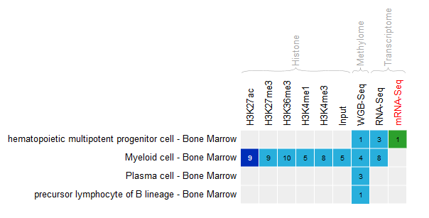
• For this exercise, we will download only two of the bigbeds for available datasets. Pick up the one for the “ERS255952” and “ERS365962” sample.

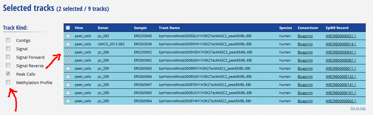
• Click “Download tracks” at the bottom of the grid.

• At the top of the download page, click on the link that says “Alternatively, you can click here to obtain a text list of all the tracks”. This will give you a text list with all tracks of interest. Copy the link to this page in your clipboard, using the address provided in your browser’s URL bar.

• Open the terminal that’s logged into Guillimin.

• Go to your module4 directory and create a place to put the material we will download.

cd ~/module4
mkdir great
cd great

• For you own analyses, you can download a bunch of tracks at the same time by using wget on a list of URLs.
  • Use the wget command to download the text file that contains the list of tracks.

wget -O trackList.txt http://epigenomesportal.ca/edcc/cgi-bin/downloadList.cgi?hubId=4580&as=1

• Now download the tracks that are contained in this list.

wget -i trackList.txt

• Convert the bigbed using the UCSC set of tools. It is available as a CVMFS module. For this example, we will convert and use only one of the files, S005HDH1.H3K27ac.ppqt_macs2_v2.20130819.bb.

module load mugqic/ucsc/20140212
bigBedToBed S005HDH1.H3K27ac.ppqt_macs2_v2.20130819.bb S005HDH1.H3K27ac.ppqt_macs2_v2.20130819.bed

Note: If you’re under Linux / Mac, you can also install the UCSC tools locally, as they are a useful set of tools to manipulate tracks data, without requiring so much processing power.

• Download the BED files locally using scp / WinSCP. Don’t forget to run the command on a local terminal session, not on Guillimin.

scp class99@guillimin.clumeq.ca:/home/class99/module4/great/*.bed .

• Load the GREAT website: http://bejerano.stanford.edu/great/public/html/

• Provide the following input to the GREAT interface:
  • Assembly: Human: GRCh37
  • One of the BED files you just downloaded.
• In the results, for instance, you should obtain something like this for biological processes:

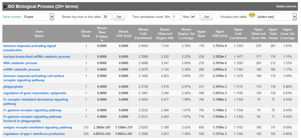
If you weren’t able to retrieve the BED file from guillimin, you can also get it here

BED file

Go back to your HOMER results

• Is the job done? (Replace %% by the number in your username)

showq -uclass%%

If the job is completed, you can bring back HOMER results to your laptop for visualiztion. From your laptop, use the scp command or WinSCP to bring back the results folder.

scp class%%@guillimin.clumeq.ca:/home/class%%/module4/homer/output .

Then, open the de novo and known motifs HTML files in a browser for visualization. Do the identified motifs fit what we would expect?

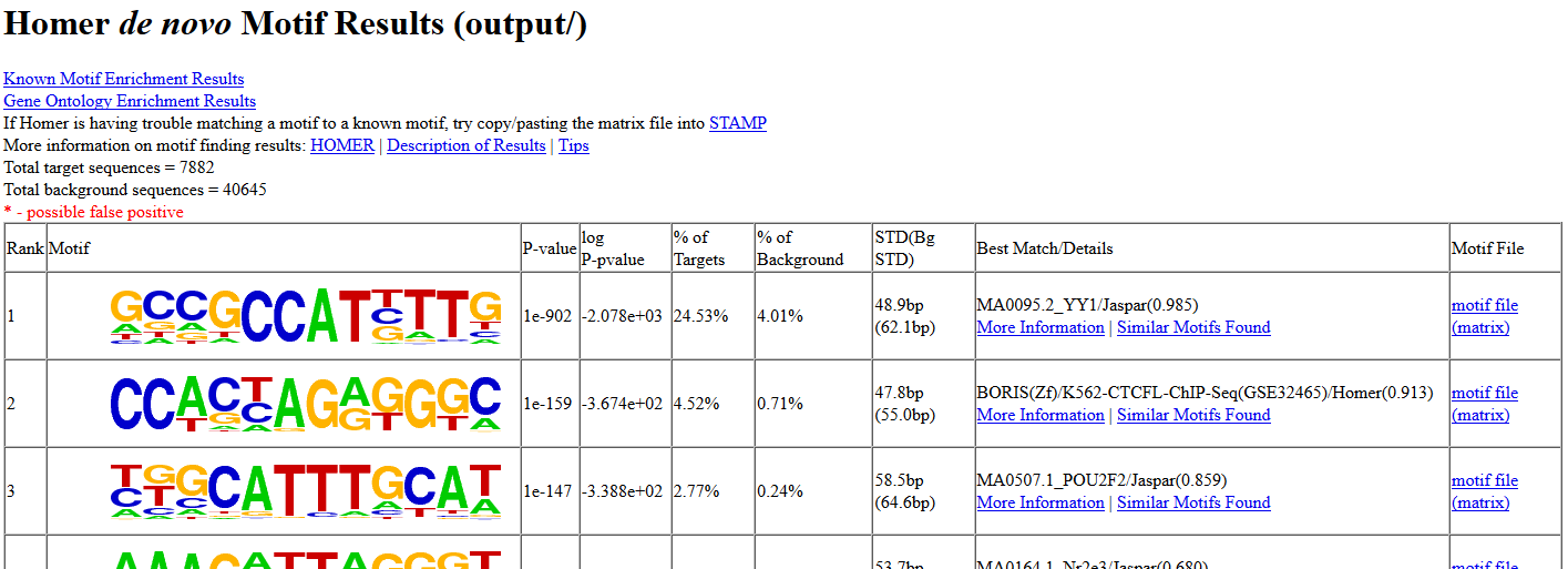
If your job didn’t complete yet, you can download the results from here instead:

Homer results

Congrats, now you’re really done!

If you have time remaining, try running queries on other types of datasets. For example, does running a GREAT query on another cell type yield the type of annotations that you’d expect?